Lab 4 displays a wide array of skill involving
Correlation and Spatial Autocorrelation. This lab helped to demonstrate skills
in Excel, putting data into it and making a scatterplot with a trend line that
is labeled in the way described. The program SPSS was also used to run
correlations, from there the correlations were put into a scatterplot and
discussed from there. Additional practice was gained in using the U.S census
website to download data and shapefiles. From the Census Data GEOID’s were
identified to help give an exact location to the data. Throughout this lab
varies data sets were joined to make help the data be easier displayed on one
map.
Part 1: Correlation
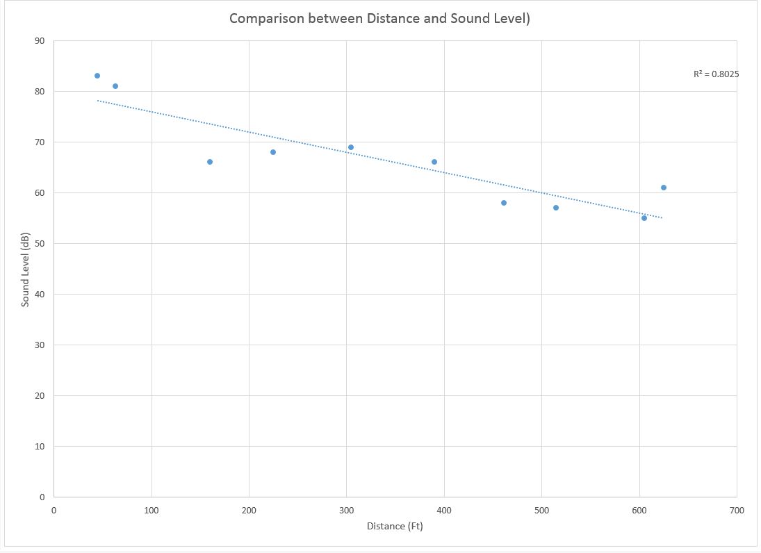
The table above shows distance in relation to sound
level. The null hypothesis states that there is no difference between distance
and sound level. There is a fairly strong negative relationship between
distance in feet and sound level in decibels. As the distance away increases
the sound level goes down. There is a significance level that would make us
nearly 100% sure that there is a negative correlation between the distance and
sound. There is a Pearson correlation of -.896, this says that there is in fact
a negative correlation between distance and sound.
 |
| Table 1: Correlation between Distance in Feet and Sound level in Decibels |
 |
| Scatterplot 1: Comparison Between Distance and Sound Level |
Part 2: Census Tracts and Population
in Detroit, MI
For part 2 there is a correlation
matrix that displays what how various ethnicities relate to one another. There
are several categories such as Median household income, if they have a bachelor’s
degree, median home value, and number that work in manufacturing, retail and
finance. The four ethnicities that are in the matrix are White, Black, Asian, Hispanic.
The median home value is highest for Whites, then Asian, followed by Blacks and
Hispanics. The trend listed about goes the same for number of people with bachelor’s
degrees, and median household income.
The Matrix does a good job of
showing how the education and incomes are very different when looking at
different ethnicities. What can be inferred is that generally speaking Whites
tend to be the wealthiest, then Asian, Black and Last Hispanics.
 |
| Table 2: Correlations between Ethnicity in Detroit Michigan |
Part 3: Spatial Autocorrelation
Introduction:
In this section data from the 1980 and 2012 elections is available from the
Texas Election Commission (TEC). The data that is given is the percent of
Democratic votes for both elections as well as the amount that voted for each
election. The TEC wants to know if there is a pattern throughout the state of
which demographic votes which way and if it has changed over the 32 year span. Throughout
this lab many skills were used in determining if there is a difference between
the voting from 1980 to 2012. In order to determine the differences GeoDa and
SPSS were both used to create scatterplots showing Moran’s I and LISA maps
displaying if there was a high-high, low-low, low-high or high-low
relationship. The TEC wants to know if there is voting patterns and clusters throughout the state.
Methodology:
The first step was to go to the US Census website to obtain data on the
Hispanic Population in 2010 because it was not given. Under the advanced search
option on the left all the counties within Texas were selected along with the
Hispanic Populations for 2010. Not all of the data that was downloaded was
needed so all but one column was deleted in order for the later join to be
successful. The data was downloaded as a shapefile from the Census site and
joined in ArcMap with a Geo ID instead of a FIPS. Once the joins were complete,
the data was exported as a new shapefile that is compatible with GeoDa.
Next
once in GeoDa under file, then open project is the new shapefile from Texas.
The goal is to see if there is a spatial autocorrelation for both elections,
voter turnout and Hispanic populations. In order to do this each of the topics
had to be weighted. Under the tools tab, weight is selected and then create,
next a variable ID is added which gives the variable its own ID, Poly ID was used
as the new variable name, this step only had to be done once. Once this weight
was created the Moran’s I and LISA cluster Maps can be created.
Two types of tests were done using the data, Moran's I and LISA maps( local indicators of spatial association). To
get the Moran’s I cluster map a tool was used at the top of the screen which
represented it, after it was selected the desired variable was clicked and the
weighted that was calculated above was used. The same step was then repeated
for the remaining variables. Next came the LISA cluster maps, another icon near
the top with similar steps as the Moran’s I. The maps below display four different colors, dark red, light red, light blue and dark blue. Red being high and blue being low.
Results:
 |
Voter Turnout 1980
 |
| Voter Turnout 1980 |
|
Conclusion: There are many things that can be taken from the
LISA maps and Moran’s I. There are patterns of voting in the state of Texas.
Over the 32 year span there has been clustering throughout the state. First
when examining the Hispanic population it is easy to see that the high clusters
on the LISA maps tend to be in the southern most parts of Texas. This is obviously
because it is the area closest to Mexico. In 1980 there was a high voter
turnout in the northern part of the pan handle of Texas. Then a similar pattern
continues in 2012, though the northern area is considerably smaller than in
1980. An interesting pattern occurs when looking at the Democratic votes throughout
the state. In 1980 the south part of Texas voted the majority Democratic and
the North tended to low-low. In 2012 the votes become even more defined. More
votes shifted toward the Democrats in the South and more went low in the north.
Also from 1980 to 2012 the low democratic voters shifted more from the western
part of the state to more central.